When you’ve been devastated by a serious car accident, your focus is on the things that matter the most: family, friends, and other loved ones. Pushing paper with your insurance agent is the last place you want your time or mental energy spent. This is why Allstate, a personal insurer in the United States, is continually seeking fresh ideas to improve its claims service for the over 16 million households they protect.
Contents
- Introduction
- Business Problem
- ML Formulation of the business problem
- Business Constraint
- Dataset
- Performance Metrics
- EDA and Preprocessing
- Encoding of the data
- Modeling part
- Kaggle Private LB submission
- Future Section
- Reference
Introduction
An insurance policy/plan is a contract between an individual (Policyholder) and an insurance company (Provider). Under the contract, you pay regular amounts of money (as premiums) to the insurer, and they pay you if the sum assured on unfortunate event arises, for example, untimely demise of the life insured, an accident, or damage to a house The Allstate Corporation is an American insurance company headquartered in Northfield Township, Illinois, near Northbrook since 1967. Allstate comes under the Top 5 insurance writers in America. In 2020, 54 percent of all people in the United States were covered by some type of life insurance, according to LIMRA’s 2020 Insurance Barometer Study
Business Problem
In the past few years, the U.S insurance industry has increased tremendously, so there is no doubt that many people also claim insurance when some unfortunate event takes place.
*Identify the predicting cost of the claim, if the higher the claim is, the more severe problem is.
As a company, Allstate could identify if the claim is severe or not, If the claim is severe it could start working on it soon. So that the claim is released as soon as possible to the needed ones.
ML Formulation of the business problem
So given anonymized data of Allstate customers, which consist of 116 categorical data and 14 numerical data we want to predict the insurance claim amount.
Business Constraint
- Minimize MAE (Mean Absolute Error)
- No strict latency constraint
- Minimize large errors while predicting the Target Value
Dataset
Source: https://www.kaggle.com/competitions/allstate-claims-severity/data
The dataset which has been provided to us is completely anonymized and no additional details have been provided to us, like what each column over here signifies to us. All the categorical columns are encoded in alphabetic format and all the numerical columns are normalized between 0 and 1
3 CSV files are provided to us —
train.csv
This file contains are the data that we will use to train our machine learning model. It consists of 188K rows with 132 columns. We have 116 categorical columns and 14 numerical columns and 1 target value, which consists of the actual insurance claim value.
test.csv
Same as train.csv files, only the major difference is that the target column is missing from here and we need to build an ML model which would predict the missing target column, which later is used to evaluate our model on Allstate Claim Severity Kaggle Competition.
submission.csv
Contains the submission format for the Kaggle Competition.
Performance Metrics
In this Kaggle Competition, submissions are evaluated on the Mean Absolute Error (MAE) between the predicted target value and the actual target value.
EDA and Preprocessing
We will be doing extensive EDA on the training dataset because we need to gain a lot of insight into how our data is and what factors affect our end results.
The dataset which is provided by Allstate doesn’t have any Null values.
Looking at the ID column we can say that some of the points are removed from the dataset to create more anonymization. This random removal of the data points can be seen throughout the dataset
train['id'].values[0:20]Output:
array([ 1, 2, 5, 10, 11, 13, 14, 20, 23, 24, 25, 33, 34, 41, 47, 48, 49, 51, 52, 55], dtype=int64)
Later I categorized all the categorical columns which have only two unique values i.e A and B. After plotting the pie chart on all the two-way categorical columns, we find out that value A has the major dominance in most of the columns.
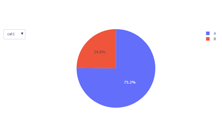
piechart on column cat1
If we take a look at our target value i.e loss column in the train.csv file
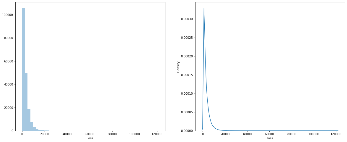
histogram and pdf on the loss column
We can see that our loss column is very skewed, to overcome this problem we will apply various transformation techniques to our loss column
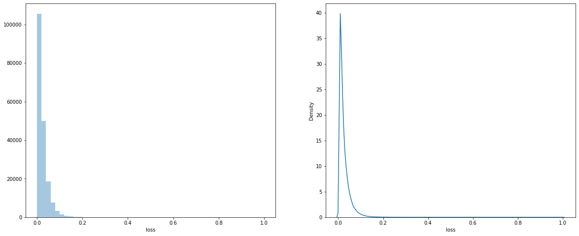
min-max transformation on loss
log transformation on loss

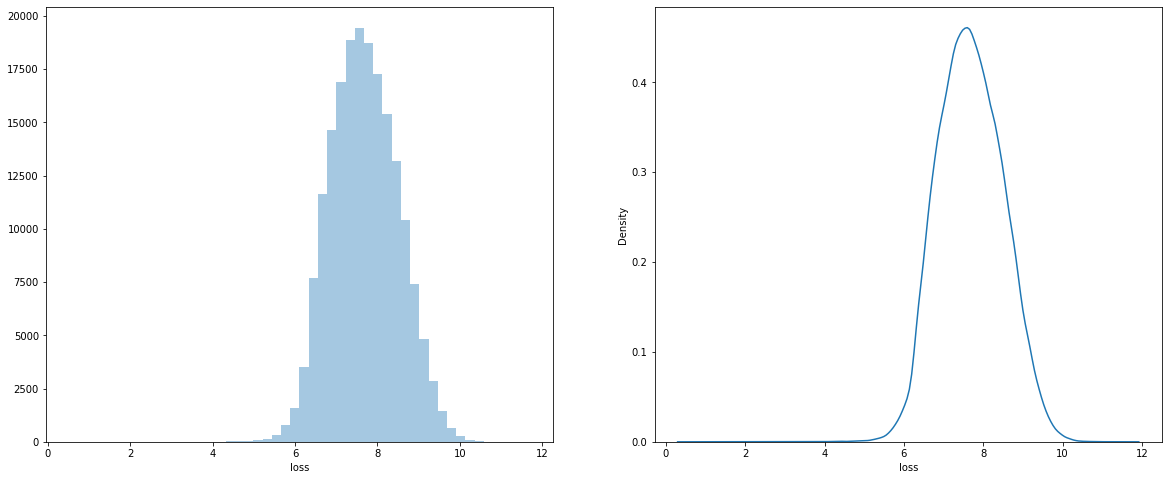
normalization + log transformation on loss
Here we can see that I applying some basic transformation functions to the loss column, the PDF of the loss column follows normal distribution now. This transformation will help our model to better learn the loss column
for i in range(0,110,10):
    print('{0} percentile - {1}'.format(i,np.percentile(train.loss_ln.values, i)))
Applying percentile on the loss column
Output:
0 percentile - 0.0
10 percentile - 0.5487345983053316
20 percentile - 0.5763245026028123
30 percentile - 0.5989953104238187
40 percentile - 0.6191047741468068
50 percentile - 0.6384448180750446
60 percentile - 0.6584707400054535
70 percentile - 0.6801497993895131
80 percentile - 0.7051612270539311
90 percentile - 0.7373587923394795
100 percentile - 1.0
If we take a look over here we can see that 0–10th percentile took a huge jump from 0.0 to 0.54, but from over there we gradually keep on increasing but for 90–100th percentile we again see that it jumped a lot between 90th and 100th percentile
Zooming in the 90–100th percentile
for i in range(90,101):
    print('{0} percentile - {1}'.format(i,np.percentile(train.loss_ln.values, i)))
Output:
90 percentile - 0.7373587923394795
91 percentile - 0.7414995960777733
92 percentile - 0.7459409784296457
93 percentile - 0.7507778033597101
94 percentile - 0.7564234976101883
95 percentile - 0.7627779024742124
96 percentile - 0.770004711840892
97 percentile - 0.7783437970174782
98 percentile - 0.7898148423985144
99 percentile - 0.8071533201770725
100 percentile - 1.0
Till the 99th percentile it was increasing gradually, but after the 99th percentile, it moved a lot
NOTE — We are working on the log normalized loss variable, not on the original loss variable.
By looking at the percentile we can say that 90% of the claim values are under 0.73. Even till the 99th percentile, our loss value is under 0.85. Between 99th — 100th percentile, our loss variable jumped a lot
If we perform the same analysis on our original loss variable, it also follows the same pattern as above.
Checking for dominant variable covered percentage in a categorical column
skewed_col = []
for i in cat_name:
    temp = dict(train[i].value_counts())
    max_key = max(temp, key=temp.get)
    area_covered = (len(train[train[i] == max_key])/len(train))*100
    if area_covered >= 99:
        skewed_col.append(i)
        print('In {0} column, value {1} has covered {2}% of area'.format(i,max_key,round(area_covered,4)))
We find out that there are 31 columns where the same value is repeated at least 99% of the time. While training our model some of the columns might not provide useful insight, so to reduce computation usage we could drop some of the columns.
While doing further analysis on the two-way categorical column, I have noticed that for column cat57, the mean value of loss value is a bit different for both the class i.e A and B. We could use this column to come up with simple and useful Feature engineer to improve the performance of our model
extracted_column = []
for i in temp_cat_list:
    if i not in skewed_col:
        temp_val = []
        for j in sorted(train[i].unique()):
            temp_df = train[train[i] == j]
            mean_value = temp_df['loss'].mean()
            mean_loss = temp_df['loss_ln'].mean()
            temp_val.append(mean_loss)
        if abs(temp_val[1] - temp_val[0]) >= 0.10:
            extracted_column.append(i)
            print('#'*25)
            print('In {0} column - {1}, its mean value is {2}'.format(i,'A',temp_val[0]))
            print('In {0} column - {1}, its mean value is {2}'.format(i,'B',temp_val[1]))
            print('#'*25)
Output:
#########################
In cat57 column - A, its mean value is 0.6389277650810136
In cat57 column - B, its mean value is 0.766728360555299
#########################
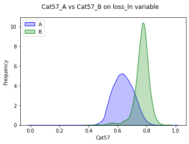
PDF on cat57 column
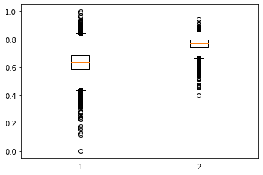
Boxplot on cat57 column
Now we are focusing on the k-way categorical column, where the categorical column can have more than 2 unique values.
#Checking dominanting variable covered percentage in categorical column
skewed_col = []
more_columns = [x for x in cat_name if len(train[x].unique()) > 2]
for i in more_columns:
    temp = dict(train[i].value_counts())
    max_key = max(temp, key=temp.get)
    area_covered = (len(train[train[i] == max_key])/len(train))*100
    if area_covered >= 99:
        skewed_col.append(i)
        print('In {0} column, value {1} has covered {2}% of area'.format(i,max_key,round(area_covered,4)))
Output:
In cat77 column, value D has covered 99.5672% of area
In cat78 column, value B has covered 99.0484% of area
We can drop the cat77 and cat78 columns in the data preprocessing stage as the data in these two columns is very skewed.
Numerical Column correlation heatmap
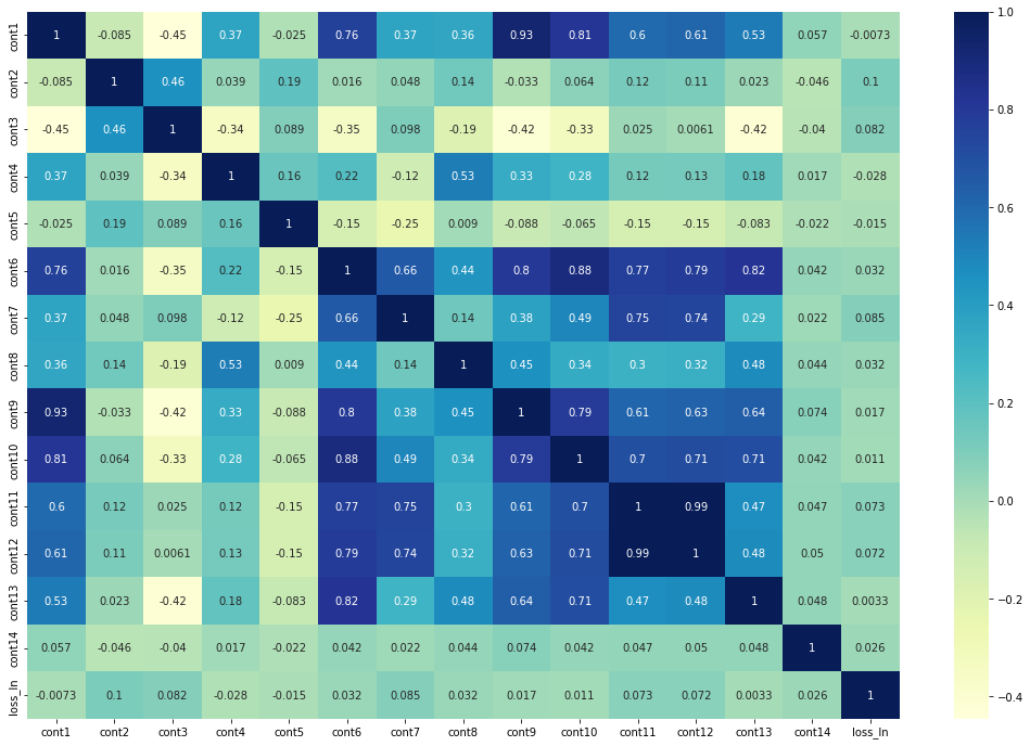
Over here we can see that cont1 and cont9 are highly correlated, same with the cont11 and cont12. There are also many other highly correlated pairs that I have not mentioned over here, while going through the preprocessing stage we need to handle all these pairs also.
Checking skewness of numerical column
for i in cont_name:
    temp = train[i].skew()
    if abs(temp) >= 1:
        print('We noticed highed skewness for {0} i.e {1}'.format(i,temp))
Output:
We noticed highed skewness for cont9 i.e 1.072428719811583
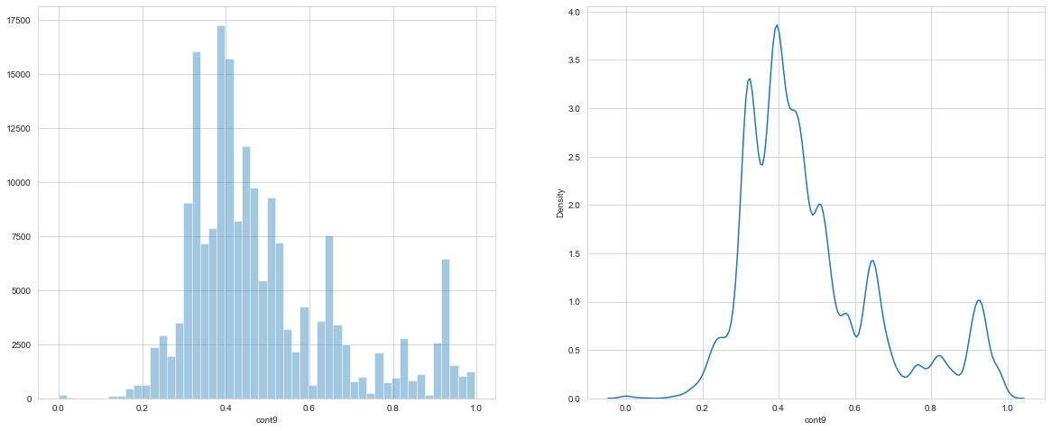
hist and PDF for cont9 column
So at the data preprocessing step, we can drop the cont9 from our dataset or we can try to apply various feature transformations to this column.
Encoding of the Data
For all the numerical columns we have applied Box Cox Transformation.
#Applying BOX-COX transformation to All numerical columns
for i in cont_name:
    data[i], fitted_lambda = stats.boxcox(data[i] + 1)
For the categorical columns, we have encoded the data using Lexical encoding.
#Applying lexical encoding to all categorical data
def lexical_encoding(charcode):
    r = 0
    ln = len(str(charcode))
    for i in range(ln):
        r += (ord(str(charcode)[i]) - ord('A') + 1) * 26 ** (ln - i - 1)
    return r

#Lexical Encoding on Categorical Data
for i in tqdm(cat_name):
    data[i] = data[i].apply(lexical_encoding)
To reduce the training time and computational usage, we have dropped some of the categorical columns where the same value is repeated at least 99.9% of the time.
#Removing all the columns where same value is repeated for 99.9% of time
zero_variance = {}
for i in cat_name:
    val_counts = dict(data[i].value_counts())
    max_key = max(val_counts, key=val_counts.get)

    var = val_counts[max_key]/len(data[i].values)
    if var >= 0.999:
        zero_variance[i] = var

data = data.drop(zero_variance.keys(), axis = 1)
cat_name = [x for x in cat_name if x not in zero_variance.keys()]
drop_col = list(zero_variance.keys())
print(drop_col)
Output:
[‘cat15’, ‘cat22’, ‘cat55’, ‘cat56’, ‘cat62’, ‘cat63’, ‘cat64’, ‘cat68’, ‘cat70’]
We have applied various types of transformation to the loss column to improve the performance of our model
#Applying normaliztion to loss column
loss_log = np.log(target['loss'] + 1)
target['normalized_log_loss'] = (loss_log-loss_log.min())/(loss_log.max()-loss_log.min())

#Log tansformation plus shifting its value by 200
target['log_200'] =  np.log(target['loss'] + 200)

#Loss tansformation
target['loss_tranform'] = target['loss']**0.25

#Loss Transformation - (1 + loss)**0.25
target['log_loss_transform'] = (1 + target['loss'])**0.25

#Log tansformation plus shifting its value by 200
target['log_100'] =  np.log(target['loss'] + 100)

#Dividing by 10
target['loss_d10'] =  10/target['loss']

#Dividing by 10 and appying log
target['log_d10'] =  np.log(10/target['loss'])

#Loss tansformation
target['loss_tranform_50'] = target['loss']**0.5

#Loss Transformation - (1 + loss)**0.50
target['log_loss_transform_50'] = np.log((1 + target['loss'])**0.50)
Here is all the decoding function to revert the predicted value to the original loss range.
#All the decoding function which will revert back our transformed loss value to original loss value
def decode_normalized_log_loss(data):
    lmin, lmax = 0.5128236264286637, 11.703655322715969
    denormalized = data * (lmax - lmin) + lmin
    return np.exp(denormalized) - 1

def decode_log_200(data):
    return np.exp(data)-200

def decode_loss_tranform(data):
    return data**(1/float(0.25))

def decode_log_loss_transform(data):
    return data**(1/float(0.25)) - 1

def decode_log_100(data):
    return np.exp(data) - 100

def decode_loss_d10(data):
    return 10/data

def decode_log_d10(data):
    return 10/np.exp(data)

def decode_loss_tranform_50(data):
    return data**(1/float(0.50))

def decode_log_loss_transform_50(data):
    data = np.exp(data)
    return data**(1/float(0.50)) - 1
I have split the training data into two parts i.e train and val data in an 80:20 ratio. To make sure that both the train and val data follow the same loss column distribution, we have used the percentile data to bin the loss data and split it using stratifies binned data.
all_bin = [np.percentile(np.abs(target['loss']),i) for i in range(0,100)]
def bin_type(value):
    for i in range(len(all_bin)):
        if value <= all_bin[i]:
            return i


target['binned'] = target['loss'].apply(np.abs).apply(bin_type).fillna(100.0)
target = target[target['binned'] != 0.0]
data = data.loc[target.index]
X_train, X_test, y_train, y_test = train_test_split(data, target, test_size=0.10, random_state=random_state,stratify=target['binned'])
Checking the PDF of both train and val datasets.
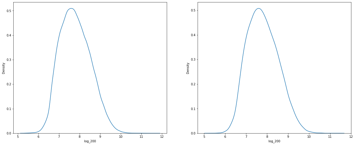
Modeling part
Here is the list of models which I have tried
- Linear Regression
- DecisionTreeRegressor
- LinearSVR
- GBDT
- XGboost
- Catboost
- LightGBM
After training all the models and testing the result on val dataset, we found that Gradient Boost Trees-based model gave us the best result. As a result, XGBoost, CatBoost, LightGBM, and GBDT gave us the best result.
So we focus more on these sets of models only.
After digging around a bit on the Kaggle Discussion forum, I found that there’s a Xgboost-based python library- XGBfir, that will use the XGboost model and give us the two-way interaction between the columns, based on which we can create new features.
#Training a XGBoost model, to retrieve two feature interaction using xgbfir library
xgb = xgboost.XGBRegressor(tree_method='gpu_hist',n_jobs=-1,random_state=random_state,seed=random_state)
xgb.fit(X_train,y_train['log_loss_transform'])
xgbfir.saveXgbFI(xgb, cat_name + cont_name, 'xgb_hist.xlsx')
XGBfir library will save the result in an Excel file. So based on this 2-way feature interaction we could create new features by performing simple operations such as addition, subtraction, or concatenation between two columns.
#Here I am concatenating and adding two way feature interaction columns
#After concatenation, I am converting all those value as int value
#Using this concatenation features, mae score of xgboost decrease quite a bit (This was confirmed using 10-fold CV and default XGBRegressor model)
data_ = data.copy()
for i in tqdm(two_way):
    features = i.split('|')
    concat_name = i.replace('|','_')
    mul_name = i.replace('|','*')
    data_[concat_name] = data_[features[0]].astype(str) + data_[features[1]].astype(str)
    data_[concat_name] = data_[concat_name].astype(int)
    data_[mul_name] = data_[features[0]].astype(float) + data_[features[1]].astype(float)
By default, the XGBoost library will evaluate our model on RMSE, but in this case, we are primarily dealing with the MAE score. So while training the XGBoost we could pass a custom metric to our XGBoost thus it will reduce our XGBoost model to make large prediction errors.
#Defining the custom objective function for xgboost model which take cares for rmse and mae
def obj(preds, dtrain):
    labels = dtrain.get_label()
    c = 1.5
    x = preds - labels
    grad = c * x /(np.abs(x) + c)
    hess = c ** 2 / (np.abs(x) + c) ** 2
    grad_rmse = x
    hess_rmse = 1.0
    grad_mae = np.array(x)
    grad_mae[grad_mae > 0] = 1.
    grad_mae[grad_mae <= 0] = -1.
    hess_mae = 1.0
    coef = [0.7, 0.15, 0.15]
    return coef[0] * grad + coef[1] * grad_rmse + coef[2] * grad_mae, coef[0] * hess + coef[1] * hess_rmse + coef[2] * hess_mae

#Over here I am evaluating model on mse score, as it helps to reduce error on bigger loss value
def xg_eval_mae(yhat, dtrain):
    y = dtrain.get_label()
    return 'mse', mae(decode_log_loss_transform(y),decode_log_loss_transform(yhat))
For hyper tuning parameter tuning of all the models, we have opted to go with Optuna. Optuna internally uses Bayesian optimization to find good parameters for our model. There’s also a big advantage of using Optuna compared to Sklearn’s GridSearchCV or RandomSearchCV. We could even run the trial search from the last point where it stopped, which is a huge plus point in the case of Optuna.
Both XGBoost and LightBGM internally support GPU boost up, so this helps us to train our model faster and efficiently.
Here are all the hyperparameter tuned values for all the models.
xgb1_params = {'n_estimators': 5500,
          'max_depth': 11,
          'min_child_weight': 100,
          'subsample': 0.9,
          'colsample_bytree': 0.9,
          'colsample_bylevel': 0.55,
          'learning_rate': 0.005,
          'base_score': 0.9,
          'tree_method':'gpu_hist',
          'n_jobs':-1,
          'seed':0,
          'random_state':random_state,
          'eval_metric': obj}

xgb2_params = {'n_estimators': 6000,
          'max_depth': 11,
          'min_child_weight': 150,
          'subsample': 0.9,
          'colsample_bytree': 0.9,
          'colsample_bylevel': 0.55,
          'learning_rate': 0.005,
          'base_score': 0.9,
          'tree_method':'gpu_hist',
          'n_jobs':-1,
          'seed':0,
          'random_state':random_state,
          'eval_metric': obj}

xgb3_params = {'n_estimators': 5500,
          'max_depth': 11,
          'min_child_weight': 100,
          'subsample': 0.9,
          'colsample_bytree': 0.9,
          'colsample_bylevel': 0.55,
          'learning_rate': 0.005,
          'base_score': 0.9,
          'tree_method':'gpu_hist',
          'n_jobs':-1,
          'seed':0,
          'random_state':random_state,
          'eval_metric': obj}

lgbm_params = {'subsample': 0.7732241782273651,
          'colsample_bytree': 0.8208793491586571,
          'min_child_samples': 119,
          'n_estimators': 1664,
          'learning_rate': 0.08833099322191373,
          'objective':'regression_l1',
Rather than using a Mean Average score of all the models, we have opted to combine all the models using Sklearn’s StackingRegressor, where we are passing all the hyper tuned models as the base model to the StackingRegressor and for the second stage, we are using CatBoostRegressor as our final predictor.
estimator = StackingRegressor([('xgb1',xgboost.XGBRegressor(**xgb1_params)),
                               ('xgb2',xgboost.XGBRegressor(**xgb2_params)),
                               ('xgb3',xgboost.XGBRegressor(**xgb3_params)),
                               ('lgbm',lightgbm.LGBMRegressor(**lgbm_params))]
                               , final_estimator = catboost.CatBoostRegressor(),
                               passthrough=True)
estimator.fit(data_,target['log_200'])
Kaggle Private LB submission
Using this model on the Kaggle test dataset, resulting in a score of 1120.53 on Public Leaderboard.

Kaggle Leaderboard submission
I have also deployed this model on my local system using Flask API.
Video Demo of the deployment —
Future Section
We can improve this model furthermore by doing some aggressive Feature Engineering and also using some Deep Learning models at the base model of StackingRegressor. As most of the winning solutions of this Kaggle competition have used some sort of Deep Learning model.