Sarcasm detection is an important component in many natural language processing (NLP) systems, directly relevant to natural language understanding, dialogue systems, and text mining. However, detecting sarcasm is difficult because it occurs infrequently and is difficult for even humans to discern.

Contents
- Introduction
- Business Problem
- ML Formulation of the business problem
- Business Constraint
- Dataset
- Performance Metrics
- EDA and Preprocessing
- Encoding of the data
- Modeling part
- Future Section
- Reference
Introduction
Reddit is an American social news aggregation, web content rating, and discussion website. Registered members submit content to the site such as links, text posts, images, and videos, which are then voted up or down by other members. Posts are organized by subject into user-created boards called “communities” or “subreddits”. Submissions with more upvotes appear towards the top of their subreddit and, if they receive enough upvotes, ultimately on the site’s front page. Reddit administrators moderate the communities. Moderation is also conducted by community-specific moderators, who are not Reddit employees. Wikipedia
Business Problem
As of September 2021, Reddit ranks as the 19th-most-visited website in the world and 7th most-visited website in the U.S. As a result millions of comments are posted on Reddit.
The problem statement over here is that, given the comment and some other metadata, we need to build a model which could classify whether the comment is sarcastic or not. This is a binary classification task. The same problem statement could be applied to various cases such as Identity political statements, offensive statements, etc.
ML Formulation of the business problem
We have been provided one CSV file which consists of all the comments, along with some other metadata such as username, no. of upvotes and downvotes, subreddit in which it was posted, parent comment, and the UTC time and date when the comment was posted.
Given this user data, we need to predict whether the comment is sarcastic or not.
Business Constraint
- Minimize AUC
- Strict Latency constraint
- Reduce False Positive Error
Dataset
This dataset contains 1.3 million Sarcastic comments from the Internet commentary website Reddit. The dataset was generated by scraping comments from Reddit and has been manually labeled 1 if it is sarcastic else 0. The provided dataset has a balanced distribution of target labels.
2 CSV files have been provided to us —
train.csv
This file contains are the data that we will use to train our machine learning model. It consists of 1.3million rows with 10 columns.
label: 1 for sarcastic else 0
comment: reply to parent Reddit comment
author: a person who commented
subreddit: a forum dedicated to a specific topic on the website Reddit
score: no. of upvotes — (minus) no. of downvotes
ups: no. of upvotes
downs: no. of downvotes
date: commented date
created_utc: commented time in UTC zone
parent_comment: the parent Reddit comment to which sarcastic replies are made
test.csv
Same as train.csv files, only the major difference is that the label column is missing from here and we need to build an ML model which would predict the missing label column, which later is used to evaluate our model on unseen data.
Performance Metrics
We will evaluate our model using the AUC score and accuracy score metrics
EDA and Preprocessing
We will be doing extensive EDA on the training dataset because we need to gain a lot of insight into how our data is and what factors affect our end results.
The dataset which is provided to us has only 53 null values in the comments columns. We are dropping all the rows where the comments data is null.
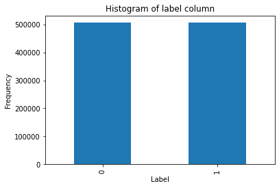
Looking at the label column we could say that, we have balanced dataset.
#plot histogram on label column
plt.title('Histogram of label column')
plt.xlabel('Label')
plt.ylabel('Frequency')
df['label'].value_counts().plot(kind='bar')
Output:
This dataset consists of scrapped data from 14,878 unique subreddit. Most of the comments are scrapped from the AskReddit subreddit channel.
df['subreddit'].value_counts()Output:
AskReddit 65677
politics 39496
worldnews 26377
leagueoflegends 21037
pcmasterrace 18988 …
LabiaGW 1
Expected 1
AnimalsStoppingFights 1
panderingfromtheright 1
Pandemic 1
Name: subreddit, Length: 14878, dtype: int64
Looking at the author’s column, we noticed that we only have 250k+ unique authors in the entire dataset, which means the dataset has multiple comments from the same authors.
len(df['author'].unique())Output:
256561
Checking out for repeated/ duplicate comments.
#Checking if any comments is duplicate
comment_counts = df['comment'].value_counts().to_dict()
#get top 10 most frequent comments
comment_counts = sorted(comment_counts.items(), key=lambda x: x[1], reverse=True)[:10]
comment_counts
Output:
[(‘You forgot the’, 1451),
(‘Yes’, 470),
(‘you forgot the’, 456),
(‘Yes.’, 456),
(‘Thanks!’, 396),
(‘You dropped this:’, 343),
(‘No.’, 342),
(‘You forgot your’, 329),
(‘You forgot’, 283),
(‘No’, 277)]
Here we can see that many came comments are repeated multiple, So at the time of data preprocessing we can drop these repeated comments, so our model doesn’t get overfit
PDF plot on no. of words in each comment
#no of words in each comment
comment_length = [len(x) for x in df['comment'].str.split(' ') if x != None]
sns.distplot(comment_length)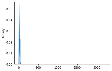
#Focusing between 0 - 250 words
comment_length = [len(x) for x in df['comment'].str.split(' ') if x != None and len(x) < 250]
sns.distplot(comment_length)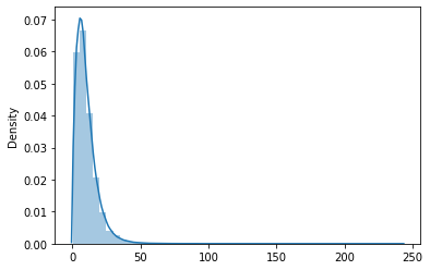
Here we can see that most of the comments have less than 50 words in them.
#Percentile on comment length
for i in range(0,110,10):
    print(i, np.percentile(comment_length, i))
Output:
0 1.0
10 3.0
20 4.0
30 6.0
40 7.0
50 9.0
60 10.0
70 12.0
80 15.0
90 20.0
100 242.0
#Percentile on comment length
for i in range(90,101):
    print(i, np.percentile(comment_length, i))
Output:
90 20.0
91 21.0
92 22.0
93 23.0
94 24.0
95 25.0
96 27.0
97 29.0
98 32.0
99 38.0
100 242.0
So at the preprocessing step, we could pad all of our sentences to 40 words, as 99% of comments have less than 38 words in them. This would result in faster training and also save us excess GPU and RAM usage.
Take a look at the score column
df['score'].min() , df['score'].max()Output:
(-507, 9070)
Over here score columns vary from -507 to 9070. Usually, the comments which are insensitive or irrelevant get downvoted on Reddit, So score could be the important factor over here.
Focusing on the Ups and Downs column
#plot sns distribuition on ups column
sns.distplot(df['ups'])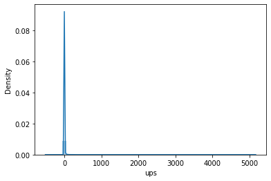
#percentile on ups column
for i in range(0,110,10):
    print(i, np.percentile(df['ups'], i))
Output:
0 -507.0
10 -1.0
20 -1.0
30 1.0
40 1.0
50 1.0
60 2.0
70 3.0
80 5.0
90 10.0
100 5163.0
Here the ups columns consist of some negative sample, which could be considered a wrong point as ups columns should only consist of positive numbers, so we could set those points as NaN or 0 at preprocessing step
#plot sns distribuition on downs column
sns.distplot(df['downs'])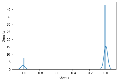
#percentile on downs column
for i in range(0,110,10):
    print(i, np.percentile(df['downs'], i))
Output:
0 -1.0
10 -1.0
20 0.0
30 0.0
40 0.0
50 0.0
60 0.0
70 0.0
80 0.0
90 0.0
100 0.0
There are no outliers present in the downs columns, as all the points are less than or equal to 0
Looking at the parent_comment column
#no of words in each parent_comment
comment_length = [len(x) for x in df['parent_comment'].str.split(' ') if x != None]
sns.distplot(comment_length)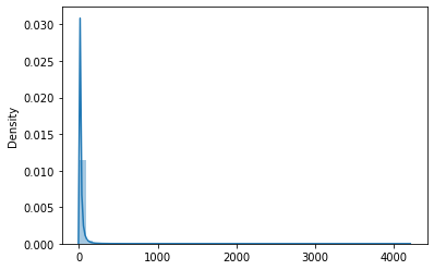
#Focusing between 0 - 500 words
comment_length = [len(x) for x in df['parent_comment'].str.split(' ') if x != None and len(x) < 500]
sns.distplot(comment_length)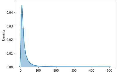
#Percentile on parent_comment length
for i in range(0,110,10):
    print(i, np.percentile(comment_length, i))
Output:
0 1.0
10 4.0
20 7.0
30 9.0
40 11.0
50 14.0
60 17.0
70 23.0
80 32.0
90 51.0
100 499.0
#distplot on label column for both classes
comment_length0 = [len(x) for x in df0['comment'].astype(str).str.split(' ') if x != None and len(x) < 250]
comment_length1 = [len(x) for x in df1['comment'].astype(str).str.split(' ') if x != None and len(x) < 250]
sns.distplot(comment_length0)
sns.distplot(comment_length1)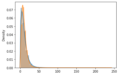
Here we could see that for both the classes the comment column follows the same distribution
Encoding of the data
First of all, I have used a stratified split to split the dataset into train, test, and val. This will make sure that each split follows the same distribution pattern.
#Checking label distribution
X_train['label'].value_counts(), X_val['label'].value_counts(), X_test['label'].value_counts()
Output:
(0 363891
1 363865
Name: label, dtype: int64,
0 40433
1 40429
Name: label, dtype: int64,
0 101081
1 101074
Name: label, dtype: int64)
To preprocess the dataset, I have converted all the major columns such as comment, author, subreddit, and parent_comment to lowercase.
#coverting string to lowercase
def string_lower(x):
    for i in ['comment','author','subreddit','parent_comment']:
        x[i] = x[i].str.lower()
    return x

X_train = string_lower(X_train)
X_val = string_lower(X_val)
X_test = string_lower(X_test)
Processing the Textual Data.
#preprocess textual data
def remove_contractions(x):
    output = []
    for i in x.split(' '):
        output.append(contractions.fix(i))
    output = ' '.join(output)
    #remove newline
    output = re.sub(r'\n', ' ', output)
    # put spaces before & after punctuations to make words seprate. Like "king?" to "king", "?"
    #code link - https://www.kaggle.com/code/prashantkikani/are-you-being-sarcastic-sarcasm-detection-nlp
    output = re.sub(r"([?!,+=—&%\'\";:¿।।।|\(\){}\[\]//])", r" \1 ", output)
    # Remove more than 2 continues spaces with 1 space.
    output = re.sub('[ ]{2,}', ' ', output).strip()
    return output

def remove_contractions_df(x):
    for i in ['comment','parent_comment']:
        x[i] = x[i].apply(remove_contractions)
    return x

X_train = remove_contractions_df(X_train)
X_val = remove_contractions_df(X_val)
X_test = remove_contractions_df(X_test)
Encoding of the data
For encoding the textual data I have used the TF2 Tokenizer function and padded it to 40 words.
#Tokenizing the data
tokenizer = tf.keras.preprocessing.text.Tokenizer(num_words=CFG.VOCAB_SIZE, oov_token='<unk>')
tokenizer.fit_on_texts(X_train['comment'])

train_data = tokenizer.texts_to_sequences(X_train['comment'])
train_data = tf.keras.preprocessing.sequence.pad_sequences(train_data, maxlen=CFG.MAX_LEN)

val_data = tokenizer.texts_to_sequences(X_val['comment'])
val_data = tf.keras.preprocessing.sequence.pad_sequences(val_data, maxlen=CFG.MAX_LEN)

test_data = tokenizer.texts_to_sequences(X_test['comment'])
test_data = tf.keras.preprocessing.sequence.pad_sequences(test_data, maxlen=CFG.MAX_LEN)
I have also used pretrained Embedding vectors over here.
GLoVE Vector
embeddings_index = {}
with open('..\\pretrained_models\\glove.840B.300d.txt', encoding='utf-8') as f:
    for line in tqdm(f):
        values = line.split(' ')
        word = values[0]
        coords = np.asarray(values[1:], dtype='float32')
        embeddings_index[word] = coords
embedding_matrix = np.zeros((len(word_index) + 1, CFG.EMBEDDING_DIM))
for word, i in word_index.items():
    embedding_vector = embeddings_index.get(word)
    if embedding_vector is not None:
        # words not found in embedding index will be all-zeros.
        embedding_matrix[i] = embedding_vector
FastText Vector
ft_path = r"..\pretrained_models\crawl-300d-2M.vec"

def get_coefs(word, *arr):
    return word, np.asarray(arr, dtype='float32')

embeddings_index = dict(get_coefs(*o.rstrip().rsplit(' ')) for o in tqdm(open(ft_path,'r',encoding='utf-8')))
word_index = tokenizer.word_index
embedding_matrix = np.zeros((len(word_index) + 1, CFG.EMBEDDING_DIM))
for word, i in tqdm(word_index.items()):
    if i >= len(word_index) + 1: continue
    embedding_vector = embeddings_index.get(word)
    if embedding_vector is not None: embedding_matrix[i] = embedding_vector
Modeling part
For the baseline model, I have built an LSTM-based model which takes tokenize comment as input. Over here I am using pre-trained embedding layers i.e GLoVE and FastText vectors.
input_layer = Input(shape=(CFG.MAX_LEN,))
embedding_layer = Embedding(input_dim=len(word_index)+1,
                            output_dim=CFG.EMBEDDING_DIM,
                            weights=[embedding_matrix],
                            input_length=CFG.MAX_LEN,
                            trainable=False)(input_layer)
lstm_layer = LSTM(100,name='LSTM')(embedding_layer)
dropout_layer = Dropout(0.2)(lstm_layer)
dense_layer_1 = Dense(units=256, activation='sigmoid')(dropout_layer)
dense_layer_2 = Dense(units=128, activation='sigmoid')(dropout_layer)
output_layer = Dense(units=1, activation='sigmoid')(dense_layer_2)

model = Model(inputs=input_layer, outputs=output_layer)
model.compile(loss=CFG.LOSS, optimizer=CFG.OPTIMIZER, metrics=['accuracy'])
I have used the same architecture for both GLoVE and FastText vector, it resulted in the following score on the Test Data.
GLoVE + LSTM: Accuracy 0.74, F1 Score 0.75
FastText + LSTM: Accuracy 0.74, F1 Score 0.75
I have also used Logistic Regression to build a baseline model. For this approach, I have encoded the textual data into the TFIDF form.
tf_idf = TfidfVectorizer(ngram_range=(1, 2), max_features=50000, min_df=2)
logit = LogisticRegression(C=1, n_jobs=-1, solver='lbfgs', random_state=17, verbose=1)
tfidf_logit_pipeline = Pipeline([('tf_idf', tf_idf),
                                 ('logit', logit)])
Logistic Regression: Accuracy 0.74, F1 Score 0.74
So we can see that Deep Learning approaches resulted in better results compared to classical Machine Learning techniques. So we will be focusing more on Deep Learning approaches.
Using the above neural network architecture but this time passing more data such as score column, as while doing EDA we found out that score column could be an important factor to improve performance of our model.
input_layer = Input(shape=(CFG.MAX_LEN,))
embedding_layer = Embedding(input_dim=len(word_index)+1,
                            output_dim=CFG.EMBEDDING_DIM,
                            weights=[embedding_matrix],
                            input_length=CFG.MAX_LEN,
                            trainable=False)(input_layer)
lstm_layer = LSTM(100,name='LSTM')(embedding_layer)
dropout_layer = Dropout(0.2)(lstm_layer)

#take score as input
input_layer2 = Input(shape=(1,),name='score_input')
dense_layer2_1 = Dense(units=256, activation='relu')(input_layer2)

#concatenate the two layers
concat_layer = Concatenate()([dropout_layer, dense_layer2_1])

dense_layer_1 = Dense(units=256, activation='relu')(concat_layer)
dense_layer_2 = Dense(units=128, activation='relu')(dense_layer_1)
output_layer = Dense(units=1, activation='sigmoid')(dense_layer_2)

model = Model(inputs=[input_layer,input_layer2], outputs=output_layer)
model.compile(loss=CFG.LOSS, optimizer=CFG.OPTIMIZER, metrics=['accuracy'])
Using the above model with both pretrained vectors.
FastText + LSTM + Score Column: Accuracy 0.72, F1 Score 0.73
tf.keras.backend.clear_session()
input_layer = Input(shape=(CFG.MAX_LEN,))
embedding_layer = Embedding(input_dim=len(word_index)+1,
                            output_dim=CFG.EMBEDDING_DIM,
                            weights=[embedding_matrix],
                            input_length=CFG.MAX_LEN,
                            trainable=False)(input_layer)
lstm_layer = LSTM(100,name='LSTM')(embedding_layer)
flatten1 = Flatten()(lstm_layer)

input_layer2 = Input(shape=(CFG.MAX_LEN,))
embedding_layer2 = Embedding(input_dim=len(word_index)+1,
                            output_dim=CFG.EMBEDDING_DIM,
                            weights=[embedding_matrix],
                            input_length=CFG.MAX_LEN,
                            trainable=False)(input_layer2)
lstm_layer2 = LSTM(100,name='LSTM2')(embedding_layer2)
flatten2 = Flatten()(lstm_layer2)

input_layer3 = Input(shape=(1,))
dense_layer1 = Dense(64, activation='relu')(input_layer3)
flatten3 = Flatten()(dense_layer1)


dropout_rate = 0.4
concat_layer = Concatenate()([flatten1, flatten2, flatten3])
dropout_layer = Dropout(dropout_rate)(concat_layer)
dense_layer_1 = Dense(512, activation='relu')(dropout_layer)
dense_layer_2 = Dense(256, activation='relu')(dense_layer_1)
output_layer = Dense(1, activation='sigmoid')(dense_layer_2)
FastText + LSTM + Extra Column: Accuracy 0.74, F1 Score 0.76
Using SOTA approaches — BERT Model
BERT is an open-source machine learning framework for natural language processing (NLP). BERT is designed to help computers understand the meaning of ambiguous language in the text by using surrounding text to establish context. The BERT framework was pre-trained using text from Wikipedia and can be fine-tuned to multiple NLP tasks.
Here we are using TPU to train our BERT model.
#Setting up TPU
try:
    tpu = tf.distribute.cluster_resolver.TPUClusterResolver()
    tf.config.experimental_connect_to_cluster(tpu)
    tf.tpu.experimental.initialize_tpu_system(tpu)
    strategy = tf.distribute.experimental.TPUStrategy(tpu)
except ValueError:
    strategy = tf.distribute.get_strategy() # for CPU and single GPU
    print('Number of replicas:', strategy.num_replicas_in_sync)
We are using a pre-trained distilbert model from huggingface library.
model_name = "distilbert-base-uncased"
tokenizer = BertTokenizer.from_pretrained(model_name)
Encoding the data from BERT architecture
def bert_encode(data):
    tokens = tokenizer.batch_encode_plus(data, max_length=CFG.MAX_LEN, padding="max_length", truncation=True)
    return tf.constant(tokens["input_ids"])


train_encoded = bert_encode(X_train['comment'])
val_encoded = bert_encode(X_val['comment'])
test_encoded = bert_encode(X_test['comment'])

train_labels = X_train.label.values
val_labels = X_val.label.values
test_labels = X_test.label.values

train_dataset = (
    tf.data.Dataset.from_tensor_slices((train_encoded, train_labels))
    .shuffle(100)
    .batch(CFG.BATCH_SIZE)
).cache()
val_dataset = (
    tf.data.Dataset.from_tensor_slices((val_encoded, val_labels))
    .shuffle(100)
    .batch(CFG.BATCH_SIZE)
).cache()
Model Architecture
def bert_model():
    bert_encoder = TFBertModel.from_pretrained(model_name, output_attentions=True)
    input_word_ids = Input(shape=(CFG.MAX_LEN,), dtype=tf.int32, name="input_ids")
    last_hidden_states = bert_encoder(input_word_ids)[0]
    lstm_layer = LSTM(100,name='LSTM')(last_hidden_states)
    dropout_layer = Dropout(0.2)(lstm_layer)
    dense_layer_1 = Dense(units=256, activation='sigmoid')(dropout_layer)
    dense_layer_2 = Dense(units=128, activation='sigmoid')(dropout_layer)
    output_layer = Dense(units=1, activation='sigmoid')(dense_layer_2)
    model = Model(inputs=input_word_ids, outputs=output_layer)
    return model

with strategy.scope():
    model = bert_model()
    model.compile(loss=CFG.LOSS, optimizer=tf.keras.optimizers.Adam(learning_rate=1e-5), metrics=["accuracy"])
    model.summary()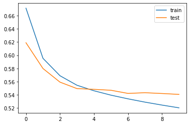
BERT loss vs val_loss
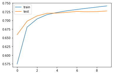
BERT accuracy vs val_accuracy
This BERT model resulted in a score of
BERT Model: Accuracy 0.77, F1 Score 0.76
I have also deployed this model on my local system using Flask API.
Video Demo of the deployment —
Future Section
We can improve this model furthermore by doing innovative text preprocessing. Our current approach uses the lighter version of the Bert Model due to the limited access to compute power. If computing power is not the issue for us, then we would use the bigger version of the BERT model.